Exercise Solutions
Model selection with the Loyn data
In the previous exercise you fitted a pre-conceived model which
included the main effects of the area of the forest patch
(LOGAREA), the grazing intensity (FGRAZE) and
the interaction between these two explanatory variables
(FGRAZE:LOGAREA). This was useful as a training exercise,
and might be a viable approach when analysing these data if the
experiment had been designed to test these effects only. However, if
other potentially important variables are not included in the model this
may lead to biased inferences (interpretation). Additionally, if the
goal of the analysis is to explore what models explain the data in a
parsimonious way (as opposed to formally testing hypotheses), we would
also want to include relevant additional explanatory variables.
Here we revisit the previous loyn data analysis, and ask if a
‘better’ model for these data could be achieved by including additional
explanatory variables and by performing model selection. Because we
would like to test the significance of the interaction between
LOGAREA, and FGRAZE, whilst accounting for the
potential effects of other explanatory variables, we will also include
LOGAREA, FGRAZE and their interaction in the
model as before. Including other interaction terms between other
variables may be reasonable, but we will focus only on the
FGRAZE:LOGAREA interaction as we have relatively little
information in this data set (67 observations). This will hopefully
avoid fitting an overly complex model which will estimate many
parameters for which we have very little data. This is a balance you
will all have to maintain with your own data and analyses (or better
still, perform a power analysis before you even collect your data). No
4-way interaction terms in your models please!
It’s also important to note that we will assume that all the explanatory variables were collected by the researchers because they believed them to be biologically relevant for explaining bird abundance (i.e. data were collected for a reason). Of course, this is probably not your area of expertise but it is nevertheless a good idea to pause and think what might be relevant or not-so relevant and why. This highlights the importance of knowing your study organism / study area and discussing research designs with colleagues and other experts in the field before you collect your data. What you should try to avoid is collecting heaps of data across many variables (just because you can) and then expecting your statistical models to make sense of it for you. As mentioned in the lecture, model selection is a relatively controversial topic and should not be treated as a purely mechanical process. Your expertise needs to be woven into this process otherwise you may end up with a model that is implausible or not very useful (and all models need to be useful!).
1. Import the ‘loyn.txt’ data file into RStudio and assign it to a
variable called loyn. Here we will be using all the
explanatory variables to explain the variation in bird density. If
needed, remind yourself of your data exploration you conducted
previously. Do any of the remaining variables need transforming
(i.e. AREA, DIST, LDIST) or
converting to a factor type variable (i.e. GRAZE)? Add the
transformed variables to the loyn dataframe.
loyn <- read.table("data/loyn.txt", header = TRUE)
str(loyn)
## 'data.frame':    67 obs. of  8 variables:
##  $ SITE   : int  1 60 2 3 61 4 5 6 7 8 ...
##  $ ABUND  : num  5.3 10 2 1.5 13 17.1 13.8 14.1 3.8 2.2 ...
##  $ AREA   : num  0.1 0.2 0.5 0.5 0.6 1 1 1 1 1 ...
##  $ DIST   : int  39 142 234 104 191 66 246 234 467 284 ...
##  $ LDIST  : int  39 142 234 311 357 66 246 285 467 1829 ...
##  $ YR.ISOL: int  1968 1961 1920 1900 1957 1966 1918 1965 1955 1920 ...
##  $ GRAZE  : int  2 2 5 5 2 3 5 3 5 5 ...
##  $ ALT    : int  160 180 60 140 185 160 140 130 90 60 ...

loyn$LOGAREA <- log10(loyn$AREA)
loyn$LOGDIST <- log10(loyn$DIST)
loyn$LOGLDIST <- log10(loyn$LDIST)

# create factor GRAZE as it was originally coded as an integer
loyn$FGRAZE <- factor(loyn$GRAZE)
2. Let’s start with a very quick graphical exploration of any
potential relationships between each explanatory variable (collinearity)
and also between our response and explanatory variables (what we’re
interested in). Create a pairs plot using the function
pairs()of your variables of interest. Hint: restrict the
plot to the variables you actually need. An effective way of doing this
is to store the names of the variables of interest in a vector
VOI <- c("Var1", "Var2", ...) and then use the naming
method for subsetting the data set Mydata[, VOI]. If you
feel like it, you can also add the correlations to the lower triangle of
the plot as you did previously (don’t forget to define the function
first).
# define the panel.cor function from ?pairs
panel.cor <- function(x, y, digits = 2, prefix = "", cex.cor, ...)
{
    usr <- par("usr")
    par(usr = c(0, 1, 0, 1))
    r <- abs(cor(x, y))
    txt <- format(c(r, 0.123456789), digits = digits)[1]
    txt <- paste0(prefix, txt)
    if(missing(cex.cor)) cex.cor <- 0.8/strwidth(txt)
    text(0.5, 0.5, txt, cex = cex.cor * r)
}

# subset the variables of interest
VOI<- c("ABUND", "LOGAREA", "LOGDIST", "LOGLDIST", "YR.ISOL", "ALT", "FGRAZE")
pairs(loyn[, VOI], lower.panel = panel.cor)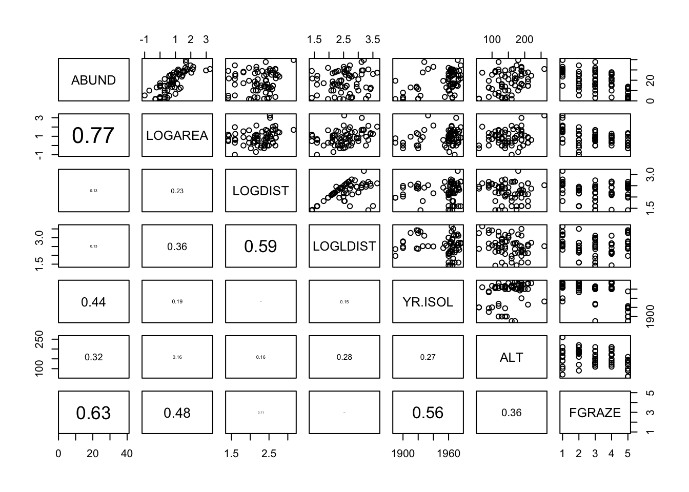
# There are varying degrees of correlation between explanatory variables which
# might indicate some collinearity, i.e. LOGAREA and FGRAZE (0.48), LOGDIST and
# LOGLDIST (0.59) and YR.ISOL and FGRAZE (0.56). However, the relationships
# between these explanatory variables are quite weak so we can probably
# include these variables in the same model (but keep an eye on things).
# There also seems to be a reasonable spread of observations across these
# pairs of explanatory variables.

# The relationship between the response variable ABUND and all the explanatory
# variables is visible in the top row:
# Some potential relationships present like with LOGAREA (positive),
# maybe ALT (positive) and FGRAZE (negative).
3. Now, let’s fit our maximal model. Start with a model of
ABUND and include all explanatory variables as main
effects. Also include the interaction LOGAREA:FGRAZE but no
other interaction terms as justified in the preamble above. Don’t forget
to include the transformed versions of the variables where appropriate
(but not the untransformed variables as well otherwise you will have
very strong collinearity between these variables!). Perhaps, call this
model M1.
M1 <- lm(ABUND ~ LOGDIST + LOGLDIST + YR.ISOL + ALT + LOGAREA + FGRAZE +
           FGRAZE:LOGAREA, data = loyn)
4. Have a look at the summary table of the model using the
summary() function. You’ll probably find this summary is
quite complicated with lots of parameter estimates (14) and P values
testing lots of hypotheses. Are all the P values less than our cut-off
of 0.05? If not, then this suggests that some form of model selection is
warranted to simplify our model.
summary(M1)
##
## Call:
## lm(formula = ABUND ~ LOGDIST + LOGLDIST + YR.ISOL + ALT + LOGAREA +
##     FGRAZE + FGRAZE:LOGAREA, data = loyn)
##
## Residuals:
##     Min      1Q  Median      3Q     Max
## -14.976  -1.972   0.142   2.388  10.631
##
## Coefficients:
##                   Estimate Std. Error t value Pr(>|t|)
## (Intercept)      33.963217  93.824477   0.362  0.71880
## LOGDIST           0.882214   2.204341   0.400  0.69061
## LOGLDIST         -0.253543   1.709295  -0.148  0.88264
## YR.ISOL          -0.008283   0.047374  -0.175  0.86186
## ALT               0.016979   0.018630   0.911  0.36622
## LOGAREA           3.733668   1.914379   1.950  0.05643 .
## FGRAZE2          -6.757424   4.132084  -1.635  0.10790
## FGRAZE3         -12.488020   4.542801  -2.749  0.00816 **
## FGRAZE4         -16.133695   4.838990  -3.334  0.00157 **
## FGRAZE5         -17.191221   4.991340  -3.444  0.00113 **
## LOGAREA:FGRAZE2   4.877440   2.565757   1.901  0.06275 .
## LOGAREA:FGRAZE3   9.410212   3.223378   2.919  0.00514 **
## LOGAREA:FGRAZE4  14.166912   4.304081   3.292  0.00178 **
## LOGAREA:FGRAZE5   2.617845   3.347001   0.782  0.43761
## ---
## Signif. codes:  0 '***' 0.001 '**' 0.01 '*' 0.05 '.' 0.1 ' ' 1
##
## Residual standard error: 5.009 on 53 degrees of freedom
## Multiple R-squared:  0.8034, Adjusted R-squared:  0.7551
## F-statistic: 16.66 on 13 and 53 DF,  p-value: 2.644e-14
5. Let’s perform a first step in model selection using the
drop1() function and use an F test based model
selection approach. This will allow us to decide which explanatory
variables may be suitable for removal from the model. Remember to use
the test = "F" argument to perform F tests when
using drop1(). Which explanatory variable is the best
candidate for removal and why? What hypothesis is being tested when we
do this model selection step?
# Wait: why can't we use information from the 'summary(M1)' or 'anova(M1)' functions
# to do this?

# the 'summary' table tests if the coefficient for each explanatory variable
# is significantly different from zero.

# the 'anova' tests for the significance of the proportion of variation explained
# by a particular term in the model.

# The ANOVA table also allows testing the overall significance of a categorical explanatory
# variable (like FGRAZE) which involves several parameters together (one for each level),
# which is quite is handy. But the results of this ANOVA are based on sequential
# sums of squares and therefore the order of the variables in the model
# (which is arbitrary here) matters.

# We could change the order but there are too many possible permutations.
# Summary P values don't suffer from this problem but tests different hypotheses.
# It would be useful to use an ANOVA that doesn't depend on the order
# of inclusion of the variables, this is effectively what 'drop1' does.

drop1(M1, test = "F")
## Single term deletions
##
## Model:
## ABUND ~ LOGDIST + LOGLDIST + YR.ISOL + ALT + LOGAREA + FGRAZE +
##     FGRAZE:LOGAREA
##                Df Sum of Sq    RSS    AIC F value   Pr(>F)
## <none>                      1329.8 228.20
## LOGDIST         1      4.02 1333.8 226.40  0.1602 0.690605
## LOGLDIST        1      0.55 1330.3 226.23  0.0220 0.882644
## YR.ISOL         1      0.77 1330.6 226.24  0.0306 0.861862
## ALT             1     20.84 1350.6 227.24  0.8306 0.366220
## LOGAREA:FGRAZE  4    405.04 1734.8 238.02  4.0358 0.006259 **
## ---
## Signif. codes:  0 '***' 0.001 '**' 0.01 '*' 0.05 '.' 0.1 ' ' 1

# LOGLDIST is the least significant (p = 0.88), and therefore makes the least
# contribution to the variability explained by the model, with respect to
# the number of degrees of freedom it uses (1)
6. Update and refit your model and remove the least significant
explanatory variable (from above). Repeat single term deletions with
drop1() again using this updated model. You can update the
model by just fitting a new model without the appropriate explanatory
variable and assign it to a new name (M2). Alternatively
you can use the update() function instead. I’ll show you
both ways in the solutions below.
# new model removing LOGLDIST
M2 <- lm(ABUND ~ LOGDIST + YR.ISOL + ALT + LOGAREA + FGRAZE +
           LOGAREA:FGRAZE, data = loyn)

# or use a shortcut with the update() function:
M2 <- update(M1, formula = . ~ . - LOGLDIST) # "." means all previous variables

# now redo drop1() on the new model
drop1(M2, test = "F")
## Single term deletions
##
## Model:
## ABUND ~ LOGDIST + YR.ISOL + ALT + LOGAREA + FGRAZE + LOGAREA:FGRAZE
##                Df Sum of Sq    RSS    AIC F value   Pr(>F)
## <none>                      1330.3 226.23
## LOGDIST         1      3.64 1334.0 224.41  0.1478 0.702134
## YR.ISOL         1      0.78 1331.1 224.27  0.0317 0.859332
## ALT             1     22.24 1352.6 225.34  0.9029 0.346233
## LOGAREA:FGRAZE  4    406.74 1737.1 236.10  4.1275 0.005451 **
## ---
## Signif. codes:  0 '***' 0.001 '**' 0.01 '*' 0.05 '.' 0.1 ' ' 1

# YR.ISOL is now the least significant (p = 0.859), hence makes the least
# contribution to the variability explained by the model,
# with respect to the number of degrees of freedom it uses (1)
7. Again, update the model to remove the least significant
explanatory variable (from above) and repeat single term deletions with
drop1().
M3 <- update(M2, formula = . ~ . - YR.ISOL)

drop1(M3, test = "F")
## Single term deletions
##
## Model:
## ABUND ~ LOGDIST + ALT + LOGAREA + FGRAZE + LOGAREA:FGRAZE
##                Df Sum of Sq    RSS    AIC F value   Pr(>F)
## <none>                      1331.1 224.27
## LOGDIST         1      3.28 1334.4 222.43  0.1355 0.714237
## ALT             1     25.33 1356.5 223.53  1.0468 0.310729
## LOGAREA:FGRAZE  4    405.99 1737.1 234.10  4.1936 0.004916 **
## ---
## Signif. codes:  0 '***' 0.001 '**' 0.01 '*' 0.05 '.' 0.1 ' ' 1

# LOGDIST now the least significant (p = 0.714) and should be removed from
# the next model.
8. Once again, update the model to remove the least significant
explanatory variable (from above) and repeat single term deletions with
drop1().
M4 <- update(M3, formula = . ~ . - LOGDIST)
drop1(M4, test = "F")
## Single term deletions
##
## Model:
## ABUND ~ ALT + LOGAREA + FGRAZE + LOGAREA:FGRAZE
##                Df Sum of Sq    RSS    AIC F value   Pr(>F)
## <none>                      1334.4 222.43
## ALT             1     22.84 1357.2 221.57  0.9584 0.331805
## LOGAREA:FGRAZE  4    408.56 1743.0 232.33  4.2864 0.004273 **
## ---
## Signif. codes:  0 '***' 0.001 '**' 0.01 '*' 0.05 '.' 0.1 ' ' 1

# ALT is not significant (p = 0.331)
9. And finally, update the model to remove the least significant
explanatory variable (from above) and repeat single term deletions with
drop1().
# and finally drop ALT from the model
M5 <- update(M4, formula = . ~ . - ALT)
drop1(M5, test = "F")
## Single term deletions
##
## Model:
## ABUND ~ LOGAREA + FGRAZE + LOGAREA:FGRAZE
##                Df Sum of Sq    RSS    AIC F value  Pr(>F)
## <none>                      1357.2 221.57
## LOGAREA:FGRAZE  4     389.3 1746.6 230.47  4.0874 0.00556 **
## ---
## Signif. codes:  0 '***' 0.001 '**' 0.01 '*' 0.05 '.' 0.1 ' ' 1

# the LOGAREA:FGRAZE term represents the interaction between LOGAREA and
# FGRAZE. This is significant (p = 0.005) and so our model selection
# process comes to an end.
10. If all goes well, your final model should be
lm(ABUND ~ LOGAREA + FGRAZE + LOGAREA:FGRAZE) which you
encountered in the previous exercise. Also, you may have noticed that
the output from the drop1() function does not include the
main effects of LOGAREA or FRGRAZE. Can you
think why this might be the case?
# As the interaction between LOGAREA and FGRAZE was significant at each step of
# model selection process the main effects should be left in our model,
# irrespective of significance. This is because it is quite difficult to
# interpret an interaction without the main effects. The drop1
# function is clever enough that it doesn't let you see the P values for the
# main effects, in the presence of their significant interaction.

# Also note, because R always includes interactions *after* their main effects
# the P value of the interaction term (p = 0.005) from the model selection
# is the same as P value if we use the anova() function on our final model

# Check this:
anova(M5)
## Analysis of Variance Table
##
## Response: ABUND
##                Df Sum Sq Mean Sq  F value    Pr(>F)
## LOGAREA         1 3978.1  3978.1 167.0669 < 2.2e-16 ***
## FGRAZE          4 1038.2   259.5  10.9000 1.241e-06 ***
## LOGAREA:FGRAZE  4  389.3    97.3   4.0874   0.00556 **
## Residuals      57 1357.3    23.8
## ---
## Signif. codes:  0 '***' 0.001 '**' 0.01 '*' 0.05 '.' 0.1 ' ' 1
drop1(M5, test= "F")
## Single term deletions
##
## Model:
## ABUND ~ LOGAREA + FGRAZE + LOGAREA:FGRAZE
##                Df Sum of Sq    RSS    AIC F value  Pr(>F)
## <none>                      1357.2 221.57
## LOGAREA:FGRAZE  4     389.3 1746.6 230.47  4.0874 0.00556 **
## ---
## Signif. codes:  0 '***' 0.001 '**' 0.01 '*' 0.05 '.' 0.1 ' ' 1
11. Now that you have your final model, you should go through your model validation and model interpretation as usual. As we have already completed this in the previous exercise I’ll leave it up to you to decide whether you include it here (you should be able to just copy and paste the code). Please make sure you understand the biological interpretation of each of the parameter estimates and the interpretation of the hypotheses you are testing.
# Biologically: confirming what we already found out in the previous exercise:
# There is a significant interaction between the area of the patch and the level
# of grazing

# However, some observations are poorly predicted (fitted) using the set of
# available explanatory variables (i.e. the two very large forest patches)

# Interpretation:
# Bird abundance might increase with patch area due to populations being more
# viable in large patches (e.g. less prone to extinction),
# or perhaps because there is proportionally less edge effect in larger
# patches, and this in turn provides more high quality habitat for species
# associated with these habitat patches

# The negative effect of grazing may be due to grazing decreasing resource
# availability for birds, for example plants or seeds directly, or insects
# associated with the grazed plants. There may also be more disturbance of birds
# in highly grazed forest patches resulting in fewer foraging opportunities
# or chances to mate (this is all speculation mind you!).

# Methodologically:
# Doing model selection is difficult without intrinsic / expert knowledge
# of the system, to guide what variables to include.
# Even with this data set, many more models could have been formulated.
# For example, for me, theory would have suggested to test an interaction
# between YR.ISOL and LOGDIST (or LOGLDIST?),
# because LOGDIST will affect the dispersal of birds between patches
# (hence the colonisation rate), and the time since isolation of the patch may
# affect how important dispersal has been to maintain or rescue populations
# (for recently isolated patches, dispersal, and hence distance to nearest
# patches may have a less important effect)
OPTIONAL questions if you have time / energy / inclination!
A1. If we weren’t aiming to directly test the effect of the
LOGAREA:FGRAZE interaction statistically (i.e. test this
specific hypothesis), we could also have used AIC to perform model
selection. This time when we remove each term we are looking for the
model with the lowest AIC (remember that lower AIC values are better).
If you like, you can repeat the model selection you did above, starting
with the same most-complex model (M1) as before, but this time use the
drop1() function and perform model selection using AIC
instead (omitting the test = "F" argument), each time
removing the term that gives a model with a lower AIC.
drop1(M1)
## Single term deletions
##
## Model:
## ABUND ~ LOGDIST + LOGLDIST + YR.ISOL + ALT + LOGAREA + FGRAZE +
##     FGRAZE:LOGAREA
##                Df Sum of Sq    RSS    AIC
## <none>                      1329.8 228.20
## LOGDIST         1      4.02 1333.8 226.40
## LOGLDIST        1      0.55 1330.3 226.23
## YR.ISOL         1      0.77 1330.6 226.24
## ALT             1     20.84 1350.6 227.24
## LOGAREA:FGRAZE  4    405.04 1734.8 238.02
#Removing the term 'LOGLDIST' gives the lowest AIC of 226.23
#So refit your model with this term removed. Run `drop1()` again on your updated model. Perhaps call this new model `M2.AIC`.
M2.AIC <- update(M1, formula = . ~ . - LOGLDIST)
drop1(M2.AIC) #removing which term gives the lowest AIC?
## Single term deletions
##
## Model:
## ABUND ~ LOGDIST + YR.ISOL + ALT + LOGAREA + FGRAZE + LOGAREA:FGRAZE
##                Df Sum of Sq    RSS    AIC
## <none>                      1330.3 226.23
## LOGDIST         1      3.64 1334.0 224.41
## YR.ISOL         1      0.78 1331.1 224.27
## ALT             1     22.24 1352.6 225.34
## LOGAREA:FGRAZE  4    406.74 1737.1 236.10
#Continue in this manner until removing any terms INCREASES the AIC. Then we have our minimal adequate model (which should be the same as the final model we finished with last time)
A2. However, the “superpower” of AIC is the ability to simultaneously compare multiple competing models, something we are not taking advantage of when we perform a stepwise model selection process. So, another approach to selecting our best model is to decide which set of models we are going to compare before we fit any of them, then fit them all, extract the AIC values, and see which model(s) have the lowest.
Fit 5 different models with the following terms, giving each model appropriate names to distinguish from the other models we have fitted so far: 1) “LOGLDIST + YR.ISOL + ALT + LOGAREA + FGRAZE + LOGAREA:FGRAZE”, 2) “LOGLDIST + YR.ISOL + ALT + LOGAREA + FGRAZE + LOGLDIST:YR.ISOL + LOGAREA:FGRAZE”, 3) “YR.ISOL + LOGAREA + FGRAZE”, 4) “LOGAREA + FGRAZE + LOGAREA:FGRAZE”, 5) “LOGAREA + FGRAZE”. If you like, you can add further models using combinations of terms you think might give the best model. Which model do you think will have the lowest AIC?
#Fit each model using the terms described above, giving each a unique and sensible name
M.AIC.1<- lm(ABUND ~ LOGLDIST + YR.ISOL + ALT + LOGAREA + FGRAZE + LOGAREA:FGRAZE, data= loyn)

M.AIC.2<- lm(ABUND ~ LOGLDIST + YR.ISOL + ALT + LOGAREA + FGRAZE + LOGLDIST:YR.ISOL + LOGAREA:FGRAZE, data= loyn)

M.AIC.3<- lm(ABUND ~ YR.ISOL + LOGAREA + FGRAZE, data= loyn)

M.AIC.4<- lm(ABUND ~ LOGAREA + FGRAZE + LOGAREA:FGRAZE, data= loyn)

M.AIC.5<- lm(ABUND ~ LOGAREA + FGRAZE, data= loyn)
A3. Now we have fitted our set of models, we can calculate the AIC of
each using the AIC() function. Which has the lowest? Which
has the highest? Are there any within 2 AIC of the lowest AIC? Are there
any models that differ in a single term and have an AIC difference of
about 2? What does this tell us about the additional term?
AIC(M.AIC.1)
## [1] 418.5422
#AIC of 418.54
AIC(M.AIC.2)
## [1] 420.3372
#AIC of 420.34
AIC(M.AIC.3)
## [1] 424.5987
#AIC of 424.60
AIC(M.AIC.4)
## [1] 413.7089
#AIC of 413.71
AIC(M.AIC.5)
## [1] 422.6052
#AIC of 422.61

#So the model with the lowest AIC (= 413.71) is M.AIC.4, with the terms 'LOGAREA + FGRAZE + LOGAREA:FGRAZE'
If all goes well, the best model should be
lm(ABUND ~ LOGAREA + FGRAZE + LOGAREA:FGRAZE). This is the
same model you ended up with when using the F test based model
selection in a stepwise manner. This might not always be the case and
generally speaking AIC based model selection approaches tend to favour
more complicated minimum adequate models compared to F test
based approaches.
We don’t need to re-validate or re-interpret the model, since we have already done this previously.
I guess the next question is how to present your results from the model selection process (using either F tests or AIC) in your paper and/or thesis chapter. One approach which I quite like is to construct a table which includes a description of all of our models and associated summary statistics. Let’s do this here for the AIC based model selection, but the same principles apply when using F tests (although you will be presenting F statistics and P values rather than AIC values).
Although you can use the output from the drop1() (and do
a bit more wrangling) let’s make it a little simpler by fitting all of
our models and then use the AIC() function to calculate the
AIC values for each model rather than drop1(). Note that
the values differ slightly between the two approaches; using either is
fine but best not to mix AIC values from the drop1() and AIC()
functions.
# This is one way of constructing a summary table for reporting the results:

# create a vector of the formulas for all the models compared during our model selection (remember to add any custom models you have have added yourself!):

model.formulas<- c(
  "LOGLDIST + YR.ISOL + ALT + LOGAREA + FGRAZE + LOGAREA:FGRAZE",
  "LOGLDIST + YR.ISOL + ALT + LOGAREA + FGRAZE + LOGLDIST:YR.ISOL + LOGAREA:FGRAZE",
  "YR.ISOL + LOGAREA + FGRAZE",
  "LOGAREA + FGRAZE + LOGAREA:FGRAZE",
  "LOGAREA + FGRAZE")

#Collect the AIC values for each model (note they will be the 2nd column of the object 'model.AIC')

model.AIC = AIC(M.AIC.1, M.AIC.2, M.AIC.3, M.AIC.4, M.AIC.5) #these are the 5 models you already fitted in step A2 (plus any extra you added yourself)

# create a dataframe of models and AIC values

summary.table<- data.frame(Model = model.formulas,
    AIC= round(model.AIC[,2], 2))

# Sort the models from lowest AIC (preferred) to highest (least preferred)

summary.table<- summary.table[order(summary.table$AIC), ]

# Add the difference in AIC with respect to best model

summary.table$deltaAIC<- summary.table$AIC - summary.table$AIC[1]

# print the dataframe to the console

summary.table
##                                                                             Model    AIC deltaAIC
## 4                                               LOGAREA + FGRAZE + LOGAREA:FGRAZE 413.71     0.00
## 1                    LOGLDIST + YR.ISOL + ALT + LOGAREA + FGRAZE + LOGAREA:FGRAZE 418.54     4.83
## 2 LOGLDIST + YR.ISOL + ALT + LOGAREA + FGRAZE + LOGLDIST:YR.ISOL + LOGAREA:FGRAZE 420.34     6.63
## 5                                                                LOGAREA + FGRAZE 422.61     8.90
## 3                                                      YR.ISOL + LOGAREA + FGRAZE 424.60    10.89
Or if you prefer a prettier version to include directly in your paper
/ thesis. You will need to install the knitr package before
you can do this. See the ‘Installing R Markdown’ in Appendix A in the
Introduction to R book for more details.
| Model | AIC | deltaAIC |
|---|---|---|
| LOGAREA + FGRAZE + LOGAREA:FGRAZE | 413.71 | 0.00 |
| LOGLDIST + YR.ISOL + ALT + LOGAREA + FGRAZE + LOGAREA:FGRAZE | 418.54 | 4.83 |
| LOGLDIST + YR.ISOL + ALT + LOGAREA + FGRAZE + LOGLDIST:YR.ISOL + LOGAREA:FGRAZE | 420.34 | 6.63 |
| LOGAREA + FGRAZE | 422.61 | 8.90 |
| YR.ISOL + LOGAREA + FGRAZE | 424.60 | 10.89 |
Which model selection approach do you prefer? Can you think of pros and cons of either approach?
Whichever model selection approach you chose, what is key to remember is to perform a fully manual and thought-through model selection process, informed by the understanding of theory in the research area, and of the research questions, with rigorous model validation throughout.
End of the model selection exercise